Maskinoberoende optimering. Intermediärkod. Treadresskod.

These lecture notes are my own notes that I made in order to use during the lecture, and it is approximately what I will be saying in the lecture. These notes may be brief, incomplete and hard to understand, not to mention in the wrong language, and they do not replace the lecture or the book, but there is no reason to keep them secret if someone wants to look at them.

Idag: Maskinoberoende optimering. Intermediärkod. Treadresskod.

• ALSU-07 avsnitt 6.1, 6.2, 6.4, 6.6
• ALSU-07 avsnitt 8.4, 8.5, 9.1
• ALSU-07 avsnitt 12.1-12.2 (översiktligt)
• (ASU-86 avsnitt 8.1-8.3, 9.4, kapitel 10)
• (KP kapitel 5 och 6)

Kodoptimering ("Code Optimization")

Man menar egentligen inte "optimalt" (bästa möjliga), utan bara "bättre".

Det heter "optimization" på engelska, och "optimering" på svenska. Inte "optimisering"!

Normalt är det optimeringsfasen (-faserna) i kompilatorn som gör optimeringen, men det finns också "handoptimering", där programmeraren själv ändrar programmet. Ett exempel: i = i * 2 kan ändras till i = i << 2. Bitskiftning är en enklare operation än multiplikation, och kan på en del processorer vara snabbare.

Ett annat exempel:

    for (i = 0; i < n; ++i) {
        do_something(a[i]);
    }

    i = 0;
    while (i < n) {
        do_something(a[i]);
        ++i;
    }

    p = &a[0];
    p_after = &a[n];
    while (p != p_after) {
        do_something(*p);
        ++p;
    }

Two rules about optimization by hand:

Types of optimization:

1. Algorithms and data structures. (Ex: Change sorting algorithm, or replace a linked list with a hash table.) Best gains (from years to seconds)! Hard for the compiler, so the programmer must do it. But: SQL!
2. "Low-level" optimzation. (As above.) Better done by the compiler! (Usually. Sometimes low-level hand optimization by the programmer is both effective and required.)
3. Machine-dependent optimizations. (Register allocation, instruction choice, as in ALSU-07 chapter 8. Instruction reordering to improve pipe-lining, etc.)

Machine-dependent optimization is sometimes done using Peep-hole optimization (ALSU-07 8.7, ASU-86 9.9): Simple transformations of the generated assembly (or machine) code. Ex:

Mellankodsgenerering ("Intermediate-Code Generation")

"Intermediate code" på engelsa. "Mellankod" eller ibland "intermediärkod" på svenska.

Why generate intermediate code? Why not do everything "in the Yacc grammar"? Some reasons:

• Machine-independent optimizations on the intermediate code
• Separating the phases (modularization is good!)
• Separating front-end and back-end

Olika sorters mellankod

Some ways to represent the program:

• Trees (or DAGs)
• Three-Address Code

Graphical representations: Trees (or DAGs)

• Postfix notation is a linearized representation of a syntax tree.
• You don't need physical pointers to represent a tree!

Men: Postfixkod är svårjobbat om man ska optimera.
Exempel på infixkod: 1*(a+2)*b
I ett syntaxträd är det ganska enkelt att hitta, och optimera bort, multiplikationen med 1. (Görs i del B i labb 7.)
Postfixkoden: 1 a 2 + * b *
Svårt att hitta multiplikationen med 1 i postfixkoden! Svårt att ta bort den!

Treadresskod ("Three-Address Code")

Example: x + y * z

temp1 = y * z
temp2 = x + temp2

Treadresskod har (högst) tre adresser i varje instruktion:
var₁ = var₂ operation var₃

Note:

• Compiler-generated temporary variables (such as temp₁)
• Liknar processorns maskininstruktioner. Få processorer har en plus-gånger-instruktion, så man behöver två maskininstruktioner: multiplikationen först och additionen sen.
• Simple => Good for optimization.
• Easier to rearrange (and thus, optimize) than postfix ("stack machine") code

Treadresskod har högst tre adresser i varje instruktion. Fler typer:
var₁ = operation var₂
goto addr₁
if var₁ <= var₂ goto addr₃

Idea: Each internal node corresponds to a temp-variable!

Example: a = b * -c + b * -c (The tree in ASU-86 fig. 8.4a)

temp1 = - c
temp2 = b * temp1
temp3 = - c
temp4 = b * temp1
temp5 = temp2 + temp3
a = temp5

Types of three-address statements

1. Assignment: x = y op z (Ex: temp₅ = a + temp₄)
2. Assignment: x = op y (Ex: temp₃ = - temp₄)
3. Copy: x = y (Ex: a = temp₃)
4. Jump: goto L
5. Conditional jump: if x relop y goto L (Ex: if (temp₇ < temp₂) goto L7)
6. Procedure call: call p, n
7. Parameter for procedure call: param x
8. Return from procedure call: return y. Ex:

   param temp4
   param a
   param b
   call f, 3
   

9. Indexed assignment: x = y[z] (ex: temp₅ [ temp₄ ] = temp₉)
10. Indexed assignment: x[y] = z
11. Pointer and address operations: x = &y
12. x = *y
13. *x = y

Syntax-directed translation into three-address code

Synthesized attributes:
E.addr = the name of the temporary variable (kallades place i ASU-86)
E.code = the sequence of three-address statements that calculates the value (or they could be written to a file instead of stored in the attribute)

(Se tabellen i ALSU-07 fig. 6.19, eller i ASU-86 fig. 8.15.)

While statement (very similar to generating stack machine code, see föreläsning 9):

(Se tabellen i ALSU-07 fig. 6.36, eller i ASU-86 fig. 8.23.)

Quadruples

Skip: Also "triples" (but they are hard to optimize) and "indirect triples" (as easy to optimize as quadruples, but more complicated).

Basic Blocks and Flow Graphs

"Basic blocks" används för optimering.

Ett par termer:

• Basic block
• Flödesgraf ("flow graph")

Fler termer:

• definiera ("define") = att sätta värdet på en variabel (jämför: odefinierat värde)
• använda ("use") = att hämta värdet på en variabel
• levande ("live") = kommer (kanske) att användas mer (jfr med skräpsamling)

Transformationer på basic blocks (kort, mer sen i exemplet):

• Common subexpression elimination

  a = b + c; b = a - d; c = b + c; d = a - d;

  ->

  a = b + c; b = a - d; c = b + c; d = b;

• Dead-code elimination

  x = y + z;

  ->

  if x is dead!
• Algebraic transformations

  a = a + 0; b = b * 1; c = d ** 2;

  ->

  c = d * d;

• Interchange of statements
• Renaming temporary variables
  normal-form block: never re-use temporary variables

• Loop = den är "strongly connected" (alla noder i loopen går att nå från alla noder i loopen) samt att den har en enda ingång ("entry point")
• Inre loop ("inner loop") = en loop utan andra loopar inuti

Quicksort-exemplet

/* recursively sorts the array a, from a[m] to a[n] */
void quicksort(int m, int n) {
  int i, j;
  int v, x;
  if (n <= m)
    return;
  i = m - 1; j = n; v = a[n];
  while (1) {
    do
      i = i + 1;
    while (a[i] < v);
    do
      j = j - 1;
    while (a[j] > v);
    if (i >= j)
      break;
    x = a[i]; a[i] = a[j]; a[j] = x; /* swap */
  }
  x = a[i]; a[i] = a[n]; a[n] = x; /* swap */
  quicksort(m, j);
  quicksort(i + 1, n);
}

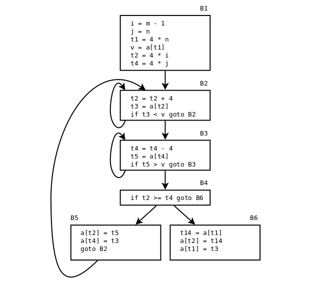
Treadresskod för den fetmarkerade delen av quicksort-funktionen (ALSU fig. 9.2 eller ASU-86 fig. 10.4):

  (1) i = m - 1                        (16) t7 = 4 * i
  (2) j = n                            (17) t8 = 4 * j
  (3) t1 = 4 * n                       (18) t9 = a[t8]
  (4) v = a[t1]                        (19) a[t7] = t9
  (5) i = i + 1                        (20) t10 = 4 * j
  (6) t2 = 4 * i                       (21) a[t10] = x
  (7) t3 = a[t2]                       (22) goto (5)
  (8) if t3 < v goto (5)               (23) t11= 4 * i
  (9) j = j - 1                        (24) x = a[t11]
 (10) t4 = 4 * j                       (25) t12 = 4 * i
 (11) t5 = a[t4]                       (26) t13 = 4 * n
 (12) if t5 > v goto (9)               (27) t14 = a[t13]
 (13) if i >= j goto (23)              (28) a[t12] = t14
 (14) t6 = 4 * i                       (29) t15 = 4 * n
 (15) x = a[t6]                        (30) a[t15] = x

Steps for the optimizer:

1. Control flow analysis: basic blocks
2. Data flow analysis.
3. Transformations.

Basic blocks och flödesgraf för quicksort-funktionen (ALSU-07 fig. 9.3 eller ASU-86 fig. 10.5):

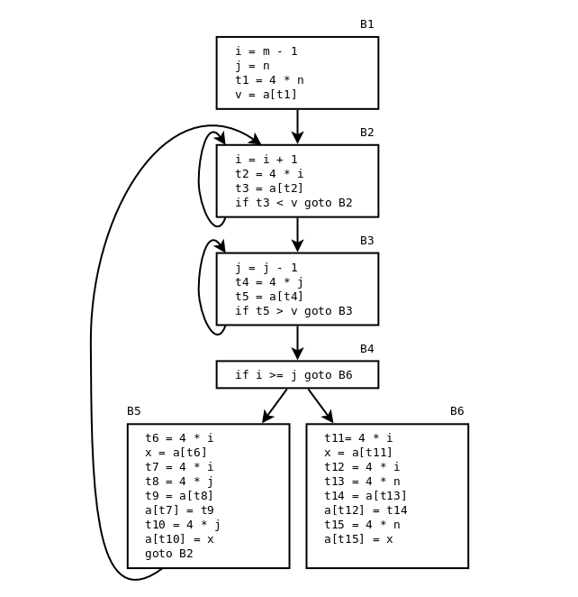
Three loops:

• B₂
• B₃
• B₂, B₃, B₄, and B₅

The principal sources of optimization

"Some of the most useful code-improving transformations".
Local transformation = inside a single basic block
Global transformation = several blocks (but inside a single procedure)

Semantics-Preserving Transformations

• Removing local common subexpressions
• Removing non-local common subexpressions
• Copy propagation
• Dead-code elimination
• ...

Removing local common subexpressions (ALSU-07 sid. 588)

t6 := 4*i
x := a[t6]
t7 := 4*i
t8 := 4*j
t9 := a[t8]
a[t7] := t9
t10 := 4*j
a[t10] := x
goto B2

t6 := 4*i
x := a[t6]
t8 := 4*j
t9 := a[t8]
a[t6] := t9
a[t8] := x
goto B2

(Remove repeat calculations, use t₆ instead of t₇, t₈ instead of t₁₀.)

Removing non-local common subexpressions (ALSU-07 9.1.4)

From ALSU-07 fig 9.4, 9.5:
(We can remove 4*i, 4*j, and 4*n completely from B₆!)
Remove 4*i and 4*j completely from B₅!

t6 := 4*i
x := a[t6]
t8 := 4*j
t9 := a[t8]
a[t6] := t9
a[t8] := x
goto B2

x := a[t2]
t9 := a[t4]
a[t2] := t9
a[t4] := x
goto B2

x := a[t2]
t9 := a[t4]
a[t2] := t9
a[t4] := x
goto B2

x := t3
t9 := a[t4]
a[t2] := t9
a[t4] := x
goto B2

Note: a hasn't changed, so a[t₄] still in t₅ from B₃

x := t3
t9 := a[t4]
a[t2] := t9
a[t4] := x
goto B2

x := t3
a[t2] := t5
a[t4] := x
goto B2

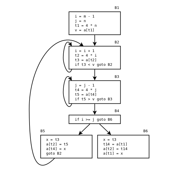
Blocken B5 och B6 efter att vi eleminerat både lokala och globala gemensamma deluttryck (ALSU-07 fig. 9.5 eller ASU-86 fig. 10.7):

Copy propagation (ALSU-07 9.1.5)

x := t3
a[t2] := t5
a[t4] := x
goto B2

x := t3
a[t2] := t5
a[t4] := t3
goto B2

Elimination of dead code (ALSU-07 9.1.6)

x := t3
a[t2] := t5
a[t4] := t3
goto B2

a[t2] := t5
a[t4] := t3
goto B2

Loop optimizations (ALSU-07 91.7-91.8)

• Move code outside the loop (so it is executed only once)
• Eliminate induction variables, that is, extra "counter variables"
• Reduce strength of operations, such as + instead of *

Examples of code motion

while (i < limit - 2)
    a[i++] = x + y;

t1 = limit - 2;
t2 = x + y;
while (i < t1)
  a[i++] = t2;

for (i = 0; i < strlen(s1); ++i)
  s2[i] = s1[i];

n = strlen(s1);
for (i = 0; i < n; ++i)
  s2[i] = s1[i];

Example of elimination of induction variables

i = 0;
j = 1;
while (a1[i] != 0) {
  a2[j] = a1[i];
  ++i;
  ++j;
}

i = 0;
while (a1[i] != 0) {
  a2[i + 1] = a1[i];
  ++i;
}

Example of both induction-variable elimination and reduction in strength

j := j-1
t4 := 4*j
t5 := a[t4]
if t5 > v goto B3

j := j-1
t4 := t4-4
t5 := a[t4]
if t5 > v goto B3

Men det där är fel, för nu får t₄ inget startvärde. Men det kan vi fixa genom att peta in t₄ = 4*j i block B₁, som körs en enda gång (inte i B₂, som körs en massa massa gånger):

ALSU-07 fig. 9.9 (ASU-86 fig 10.9):

Then a similar strength reduction of 4 * i in basic block B₂.
We know that t₂ == 4 * i. Maintain this relationship!

Then, i and j are used only in the test int B₄.
The test i >= j can be changed to 4 * t₂ >= 4 * t₄ (which is equivalent to t₂ >= t₄).
i and j become dead!

Flödesgrafen efter att vi eliminerat induktionsvariablerna i och j (ASU-86 fig 10.10 eller ALSU-07 fig. 9.9):

Exempel på en annan loop-optimering: Loop unrolling (ALSU-07 sid. 735)

for (i = 0; i < 20; ++i)
  for (j = 0; j < 2; ++j)
    a[i][j] = i + 2 * j;

for (i = 0; i < 20; ++i) {
    a[i][0] = i;
    a[i][1] = i + 2;
}

    a[0][0] = 0;
    a[0][1] = 2;
    a[1][0] = 1;
    a[1][1] = 3;
    a[2][0] = 2;
    a[2][1] = 4;
    ....
    a[19][0] = 19;
    a[19][1] = 21;

Varning: cachen! En för stor loop kanske inte får plats i processorns instruktionscache.

Exempel på en annan viktig optimering: Eliminering av svans-rekursion

void f(struct Node *p) {
    if (p == NULL)
        return;
    p->value++;
    f(p->next);
}

void f(struct Node *p) {
    while (p == NULL) {
        p->value++;
        p = p->next;
    }
}

9.2-9.10

Symbolic debugging of optimized code

int a;
...
void f(string a) {
  ...
  while (1) {
    int a;
    ...        <-- In the debugger: print a
  }
}

• (Parts) of the symbol table from compilation: the lexeme a, the type, the location in memory
• Scope information. Which a do we mean?
• Where are we, in the program? (So we can apply the scope information.)
• Some sort of mapping between source-language statements and machine code, so we know which source statement we are executing.

A program may work when unoptimized, but not when optimized. For example, the C standard specifies undefined behaviour in certain cases. such as:

char s[10];
...
s[14] = 'x';

An example program:

#include <stdlib.h> #include <stdio.h> int plus(int x, int y) { int a[2]; int s; s = x - y; a[x] = x + y; return s; } int main(void) { int resultat; resultat = plus(-1, -2); printf("resultat = %d\n", resultat); return 0; }

Running it without optimization, and then with optimization (the "-O" flag):

linux> gcc -Wall plus.c -o plus plus.c: In function 'plus': plus.c:5:9: warning: variable 'a' set but not used [-Wunused-but-set-variable] int a[2]; ^ linux> ./plus resultat = -3 linux> gcc -O -Wall plus.c -o plus plus.c: In function 'plus': plus.c:5:9: warning: variable 'a' set but not used [-Wunused-but-set-variable] int a[2]; ^ linux> ./plus resultat = 1 linux>

Trying to debug:

linux> gcc -g -O -Wall plus.c -o plus plus.c: In function 'plus': plus.c:5:9: warning: variable 'a' set but not used [-Wunused-but-set-variable] int a[2]; ^ linux> ./plus resultat = 1 linux> gdb plus Some output from GDB removed (gdb) break main Breakpoint 1 at 0x400562: file plus.c, line 12. (gdb) run Starting program: /home/padrone/tmp/14okt/plus Breakpoint 1, main () at plus.c:12 12 int main(void) { (gdb) step 15 printf("resultat = %d\n", resultat); (gdb) print resultat $1 = <optimized out> (gdb)

Deducing values of variables in basic blocks

• The variable a may have been eliminated during optimization!
• Code may have been moved by the optimizer, for example an assignment to a, so a's current value may be inconsistent with the source program!

• b + c is a common subexpression of several source-program expressions. When computed, it causes overflow and an exception.
  Where did the program crash?

ASU-86 fig 10.68. Assume that the source, intermediate and target representation are the same.

ASU-86 fig 10.69. A DAG for the variables. The DAG shows how values depend on each other. Then, annotate it with life-time information.

Example 1 (just the unoptimized program):
c = a + b after step 1. (Life time: 2-3)
c = c - e after step 3. (Life time: 4-infinity)

Example 2 (the optimized program):
c = a after step 5'. (Life time: 6'-infinty)
c is undefined in 1'-5'! (But can be calculated, differently depending on when!)

Example 3:
An overflow occurs in the optimized code, in statement 2', t = b * e.
The first source statement that uses the node b * e is 5.
Therefore, tell the user the program crashed in source statement 5!

Then the user says:

print b -> show b (lifetime 1-5 and 1'-4')
Explanation: b still has its initial value, both at 2' and at 5.

print c -> can't show actual stored c (lifetime 6-infinity)
Instead, find the DAG node for c at time 5 (-).
(Optimized) a will contain this value after 4', but not yet!
Consider the children: d contains the value from the + node at 2'-infinity. e contains the value from the E₀ node at 1'-infinity. So use d - e!

ALSU-07 kapitel 12: Interprocedural Analysis

• Skillnaden mellan intra-procedurell (engelska: intraprocedural) och inter-procedurell (engelska: interprocedural)
• Vad kan man göra med interprocedurell analys, som man inte kan göra med intraprocedurell? (Ge exempel.)
• Vad är en anropsgraf (engelska: call graph), och vad behöver man den till?
• Vad innebär pointer aliasing?
• Vad menas med procedur-inlining?

The course Compilers and interpreters | Lectures: 1 2 3 4 5 6 7 8 9 10 11 12