Det här är ungefär vad jag tänker säga på föreläsningen. Använd det för förberedelser, repetition och ledning. Det är inte en definition av kursinnehållet, och det ersätter inte kursboken.
Idag: Intermediärkod. Treadresskod. Maskinoberoende optimering.
Why generate intermediate code? Why not do everything "in the Yacc grammar"? Some reasons:
Some ways to represent the program:

Men: Postfixkod är svårjobbat om man ska optimera.
Exempel på infixkod: 1*(a+2)*b
I ett syntaxträd är det ganska enkelt att hitta, och optimera bort, multiplikationen med 1.
Postfixkoden: 1 a 2 + * b *
Svårt att hitta multiplikationen med 1 i postfixkoden! Svårt att ta bort den!
var1 = var2 operation var3
Example: x + y * z
Note:temp1 = y * z temp2 = x + temp2
Postfix: a b - a b + -
Three-Address code:
Idea: Each internal node corresponds to a temp-variable!temp1 = a - b temp2 = a + b temp3 = temp1 - temp2
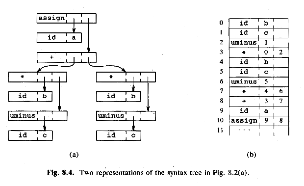
Example: a = b * -c + b * -c (The tree in ASU-86 fig. 8.4a)
The DAG in ASU-86 fig. 8.4b:temp1 = - c temp2 = b * temp1 temp3 = - c temp4 = b * temp1 temp5 = temp2 + temp3 a = temp5
temp1 = - c
temp2 = b * temp1
temp5 = temp2 + temp2
a = temp5
param temp4
param a
param b
call f, 3
Synthesized attributes:
E.addr = the name of the temporary variable
(kallades place i ASU-86)
E.code = the sequence of three-address statements that calculates the value
(or they could be written to a file instead of stored in the attribute)
| Production | Semantic rule |
|---|---|
| Start -> id = Expr | Start.code = Expr.code + [ id.addr ":=" Expr.addr ] |
| Expr -> Expr1 + Expr2 | Expr.addr = make_new_temp();
Expr.code = Expr1.code + Expr2.code + [ Expr.addr = Expr1.addr "+" Expr2.addr; ] |
| Expr -> Expr1 * Expr2 | Expr.addr = make_new_temp();
Expr.code = Expr1.code + Expr2.code + [ Expr.addr = Expr1.addr "*" Expr2.addr; ] |
| Expr -> - Expr1 | Expr.addr = make_new_temp();
Expr.code = Expr1.code + [ Expr.addr = "-" Expr1.addr; ] |
| Expr -> ( Expr1 ) | Expr.addr = Expr1.addr; // No new temp!
Expr.code = Expr1.code; |
| Expr -> id | Expr.addr = id.addr; // No temp!
Expr.code = ' '; // No code! |
(Se tabellen i ALSU-07 fig. 6.19, eller i ASU-86 fig. 8.15.)
While statement (very similar to generating stack machine code, see föreläsning 9):
| Production | Semantic rule |
|---|---|
| Stmt -> while ( Expr ) Stmt1 |
Stmt.before = make_new_label();
Stmt.after = make_new_label(); Stmt.code = [ "label" Stmt.before ] + Expr.code + [ "if" Expr.addr "==" "0" "goto" Stmt.after; ] + Stmt1.code + [ "goto" Stmt.before ] + [ "label" Stmt.after ]; |
(Se tabellen i ALSU-07 fig. 6.36, eller i ASU-86 fig. 8.23.)
| Op | Arg1 | Arg2 | result | |
|---|---|---|---|---|
| 0 | uminus | c | temp1 | |
| 1 | * | b | temp1 | temp2 |
| 2 | uminus | c | temp3 | |
| 3 | * | b | temp3 | temp4 |
| 4 | + | temp2 | temp4 | temp5 |
| 5 | := | temp5 | a |
Skip: Also "triples" (but they are hard to optimize) and "indirect triples" (as easy to optimize as quadruples, but more complicated).
"Hand optimization", example:
  for (i = 0; i < n; ++i) {
    do_something(a[i]);
  }
Equivalent to:
  i = 0;
  while (i < n) {
    do_something(a[i]);
    ++i;
  }
Can be "optimized" to:
  p = &a[0];
  p_after = &a[n];
  while (p != p_after) {
    do_something(*p);
    ++p;
  }
Probably no effect, or even slower. Better handled by the compiler!
Two rules about optimization by hand:
|
Types of optimization:
Peep-hole optimization (ALSU-07 8.7, ASU-86 9.9): Simple transformations of the generated assembly (or machine) code. Ex:
| can be changed to |
|
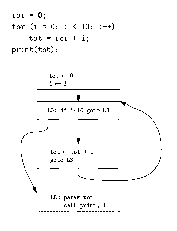
"Basic blocks" används för optimering.
Ett par termer:
Fler termer:
Transformationer på basic blocks (kort, mer sen i exemplet):
| -> |
|
| -> |
|
| -> |
|
/* recursively sorts the array a, from a[m] to a[n] */
void quicksort(int m, int n) {
  int i, j;
  int v, x;
  if (n <= m)
    return;
  i = m - 1; j = n; v = a[n];
  while (1) {
    do
      i = i + 1;
    while (a[i] < v);
    do
      j = j - 1;
    while (a[j] > v);
    if (i >= j)
      break;
    x = a[i]; a[i] = a[j]; a[j] = x; /* swap */
  }
  x = a[i]; a[i] = a[n]; a[n] = x; /* swap */
  quicksort(m, j);
  quicksort(i + 1, n);
}
Some optimizations are not possible on the source level.
ALSU fig. 9.2 (ASU-86 fig. 10.4), three-address code for a part of the quicksort function:
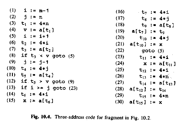
Steps for the optimizer:
ALSU-07 fig. 9.3 (ASU-86 fig. 10.5), basic blocks and flow graph for the quicksort function:
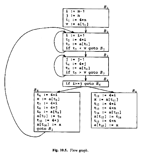
Three loops:
"Some of the most useful code-improving transformations".
Local transformation = inside a single basic block
Global transformation = several blocks (but inside a single procedure)
B5
| can be changed to |
B5
|
(Remove repeat calculations, use t6 instead of t7, t8 instead of t10.)
From ALSU-07 fig 9.4, 9.5:
(We can remove 4*i, 4*j, and 4*n completely from B6!)
Remove 4*i and 4*j completely from B5!
B5
| can be changed to |
B5
|
B5
| can then be changed to |
B5
|
Note: a hasn't changed, so a[t4] still in t5 from B3
B5
| can then be changed to |
B5
|
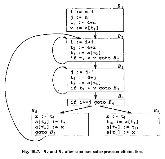
ALSU-07 fig. 9.5 (ASU-86 fig. 10.7), after eliminating (global) common subexpressions:
B5
| can be changed to |
B5
|
B5
| but x is dead, so: |
B5
|
The expressions limit - 2 and x + y are loop-invariant.while (i < limit - 2) a[i++] = x + y;
The next example is harder for the compiler, since strlen is just another function. (Or is it?)t1 = limit - 2; t2 = x + y; while (i < t1) a[i++] = t2;
for (i = 0; i < strlen(s1); ++i)
  s2[i] = s1[i];
n = strlen(s1);
for (i = 0; i < n; ++i)
  s2[i] = s1[i];
i = 0;
j = 1;
while (a1[i] != 0) {
  a2[j] = a1[i];
  ++i;
  ++j;
}
Both i and j are induction variables ("loop counters").
i = 0;
while (a1[i] != 0) {
  a2[i + 1] = a1[i];
  ++i;
}
B3
| blir |
B3
|
Men det där är fel, för nu får t4 inget startvärde. Men det kan vi fixa genom att peta in t4 = 4*j i block B1, som körs en enda gång (inte i B2, som körs en massa massa gånger):
ALSU-07 fig. 9.9 (ASU-86 fig 10.9):
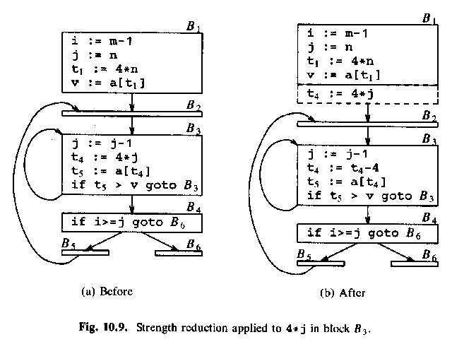
Then a similar strength reduction of 4 * i in basic block B2.
We know that t2 == 4 * i. Maintain this relationship!
Then, i and j are used only in the test int B4.
The test
i >= j
can be changed to
4 * t2 >= 4 * t4
(which is equivalent to
t2 >= t4).
i and j become dead!
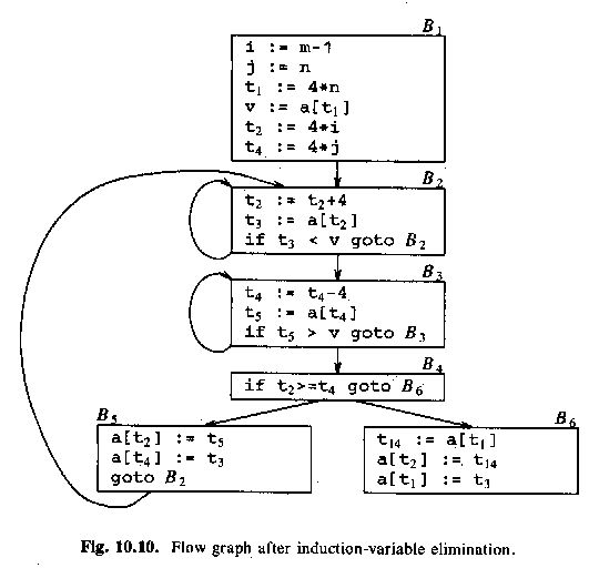
ASU-86 fig 10.10, after eliminating induction variables i and j:
for (i = 0; i < 20; ++i)
  for (j = 0; j < 2; ++j)
    a[i][j] = i + 2 * j;
may be transformed by unrolling the inner loop:
for (i = 0; i < 20; ++i) {
    a[i][0] = i;
    a[i][1] = i + 2;
}
or by unrolling the outer loop too:
    a[0][0] = 0;
    a[0][1] = 2;
    a[1][0] = 1;
    a[1][1] = 3;
    a[2][0] = 2;
    a[2][1] = 4;
    ....
    a[19][0] = 19;
    a[19][1] = 21;
Men, varning: cachen!
En för stor loop kanske inte får plats i processorns instruktionscache.
int a;
...
void f(string a) {
  ...
  while (1) {
    int a;
    ...        <-- In the debugger: print a
  }
}
What is needed, for symbolic debugging in general?
A program may work when unoptimized, but not when optimized. For example, the C standard specifies undefined behaviour in certain cases. such as:
The behaviour depends entirely on what happens to be stored at the memory location 5 bytes after the end of s: unused padding, a variable, or the return address in an activation record? This can be different with or without optimization, since optimization, for example, can eliminate variables.char s[10]; ... s[14] = 'x';
ASU-86 fig 10.68. Assume that the source, intermediate and target representation are the same.
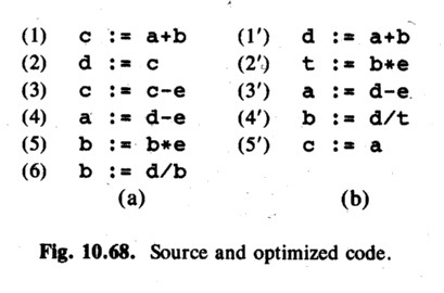
ASU-86 fig 10.69. A DAG for the variables. The DAG shows how values depend on each other. Then, annotate it with life-time information.
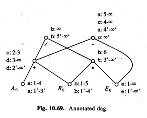
Example 1 (just the unoptimized program):
c = a + b after step 1. (Life time: 2-3)
c = c - e after step 3. (Life time: 4-infinity)
Example 2 (the optimized program):
c = a after step 5'. (Life time: 6'-infinty)
c is undefined in 1'-5'!
(But can be calculated, differently depending on when!)
Example 3:
An overflow occurs in the optimized code, in statement 2',
t = b * e.
The first source statement that uses the node b * e is 5.
Therefore, tell the user the program crashed in source statement 5!
Then the user says:
print b -> show b (lifetime 1-5 and 1'-4')
Explanation: b still has its initial value, both at 2' and at 5.
print c -> can't show actual stored c (lifetime 6-infinity)
Instead, find the DAG node for c at time 5 (-).
(Optimized) a will contain this value after 4', but not yet!
Consider the children:
d contains the value from the + node at 2'-infinity.
e contains the value from the E0 node at 1'-infinity.
So use d - e!
Kursen Kompilatorer och interpretatorer | Föreläsningar: 1 2 3 4 5 6 7 8 9 10 11 12