Kompilatorer och interpretatorer: Lecture 13

Today: Optimization.
ASU chapter 10. (KP chapter 6.)

10. Code Optimization

"Hand optimization", example:

  for (i = 0; i < n; ++i) {
    do_something(a[i]);
  }

  i = 0;
  while (i < n) {
    do_something(a[i]);
    ++i;
  }

  p = &a[0];
  p_after = &a[n];
  while (p != p_after) {
    do_something(*p);
    ++p;
  }

Two rules about optimization by hand:

1. Don't do it. (Usually not needed. If it is needed, leave it to the compiler.)
2. Don't do it yet. ("90/10 rule". Profile first!)

Types of optimization:

1. Algorithms and data structures. (Ex: Change sorting algorithm, or replace a linked list with a hash table.) Best gains (years to seconds)! Hard for the compiler. But: SQL!
2. "Low-level" optimzation. (As above.) Better done by the compiler!
3. Machine-dependent optimizations. (Register allocation, instruction choice, as in chapter 9. Instruction reordering to improve pipe-lining, etc.)

Peep-hole optimization (ASU 9.9): Simple transformations of the generated assembly (or machine) code. Ex:

10.1 Introduction

void quicksort(int m, int n) {
  int i, j;
  int v, x;
  if (n <= m)
    return;
  i = m-1; j = n; v = a[n];
  while (1) {
    do
      i = i + 1;
    while (v > a[i]);
    do
      j = j - 1;
    while (a[j] > v);
    if (i>=j)
      break;
  }
  x = a[i]; a[i] = a[n]; a[j] = x;
  quicksort(m, j);
  quicksort(i+1, n);
}

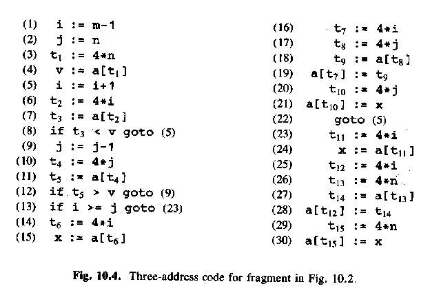
ASU fig. 10.4, three-address code for a part of the quicksort function:

Steps for the optimizer:

1. Control flow analysis: basic blocks
2. Data flow analysis.
3. Transformations.

ASU fig. 10.5, basic blocks and flow graph for the quicksort function:

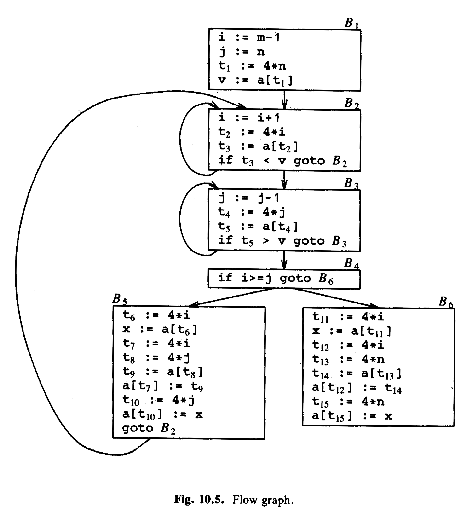
Three loops:

• B₂
• B₃
• B₂, B₃, B₄, and B₅

10.2 The principal sources of optimization

Function-preserving transformations (ASU p. 592)

B₅:

t6 := 4*i
x := a[t6]
t7 := 4*i
t8 := 4*j
t9 := a[t8]
a[t7] := t9
t10 := 4*j
a[t10] := x
goto B2

t6 := 4*i
x := a[t6]
t8 := 4*j
t9 := a[t8]
a[t6] := t9
a[t8] := x
goto B2

(Remove repeat calculations, use t₆ instead of t₇, t₈ instead of t₁₀.)

Removing (non-local) common subexpressions (ASU p. 592-594)

From fig 10.5/10.6:
(We can remove 4*i, 4*j, and 4*n completely from B₆!)
Remove 4*i and 4*j completely from B₅!

B₅:

t6 := 4*i
x := a[t6]
t8 := 4*j
t9 := a[t8]
a[t6] := t9
a[t8] := x
goto B2

x := a[t2]
t9 := a[t4]
a[t2] := t9
a[t4] := x
goto B2

x := a[t2]
t9 := a[t4]
a[t2] := t9
a[t4] := x
goto B2

x := t3
t9 := a[t4]
a[t2] := t9
a[t4] := x
goto B2

Note: a hasn't changed, so a[t₄] still in t₅ from B₃

x := t3
t9 := a[t4]
a[t2] := t9
a[t4] := x
goto B2

x := t3
a[t2] := t5
a[t4] := x
goto B2

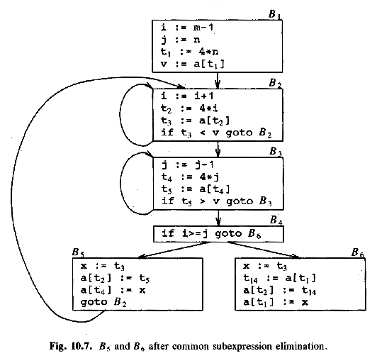
ASU fig. 10.7, after eliminating (global) common subexpressions:

Copy propagation (ASU p. 594-595)

B₅:

x := t3
a[t2] := t5
a[t4] := x
goto B2

x := t3
a[t2] := t5
a[t4] := t3
goto B2

Elimination of dead code (ASU p. 595)

B₅:

x := t3
a[t2] := t5
a[t4] := t3
goto B2

a[t2] := t5
a[t4] := t3
goto B2

Loop optimizations (ASU pp. 596-598)

• Move code
• Eliminate induction variables, that is, extra "counter variabless"
• Reduce strength of operations, such as + instead of *

Examples of code motion

while (i < limit - 2)
  a[i] = x + y;

t1 = limit - 2;
t2 = x + y;
while (i < t)
  a[i] = t2;

for (i = 0; i < strlen(s1); ++i)
  s2[i] = s1[i];

n = strlen(s1);
for (i = 0; i < n; ++i)
  s2[i] = s1[i];

Example of elimination of induction variables

i = 0;
j = 1;
while (a1[i] != 0) {
  a2[j] = a1[i];
  ++i;
  ++j;
}

i = 0;
while (a1[i] != 0) {
  a2[i + 1] = a1[i];
  ++i;
}

Example of both induction-variable elimination and reduction in strength

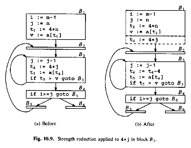
Then a similar strength reduction of 4 * i in basic block B₂.
We know that t₂ == 4 * i. Maintain this relationship!

Then, i and j are used only in the test int B₄.
The test i >= j can be changed to 4 * t₂ >= 4 * t₄ (which is equivalent to t₂ >= t₄).
i and j become dead!

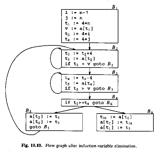
ASU fig 10.10, after eliminating induction variables i and j:

Loop unrolling

for (i = 0; i < 20; ++i)
  for (j = 0; j < 2; ++j)
    a[i][j] = i + 2 * j;

for (i = 0; i < 20; ++i) {
    a[i][0] = i;
    a[i][1] = i + 2;
}

10.3 - 10.12

10.13 Symbolic debugging of optimized code

int a;
...
void f(string a) {
  ...
  while (1) {
    int a;
    ...        <-- In the debugger: print a
  }
}

• (Parts) of the symbol table from compilation: the lexeme a, the type, the location in memory
• Scope information. Which a do we mean?
• Where are we, in the program? (So we can apply the scope information.)
• Some sort of mapping between source-language statements and machine code, so we know which source statement we are executing.

A program may work when unoptimized, but not when optimized. For example, the C standard specifies undefined behaviour in certain cases. such as:

char s[10];
...
s[14] = 'x';

Deducing values of variables in basic blocks

• The variable a may have been eliminated during optimization!
• Code may have been moved by the optimizer, for example an assignment to a, so a's current value may be inconsistent with the source program!

• b + c is a common subexpression of several source-program expressions. When computed, it causes overflow and an exception.
  Where did the program crash?

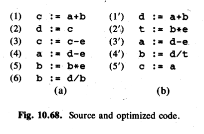
ASU fig 10.68. Assume that the source, intermediate and target representation are the same.

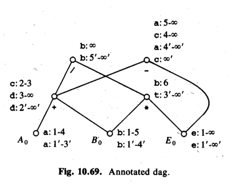
ASU fig 10.69. A DAG for the variables. The DAG shows how values depend on each other. Then, annotate it with life-time information.

Example 1 (just the unoptimized program):
c = a + b after step 1. (Life time: 2-3)
c = c - e after step 3. (Life time: 4-infinity)

Example 2 (the optimized program):
c = a after step 5'. (Life time: 6'-infinty)
c is undefined in 1'-5'! (But can be calculated, differently depending on when!)

Example 3:
An overflow occurs in the optimized code, in statement 2', t = b * e.
The first source statement that uses the node b * e is 5.
Therefore, tell the user the program crashed in source statement 5!

Then the user says:

print b -> show b (lifetime 1-5 and 1'-4')
Explanation: b still has its initial value, both at 2' and at 5.

print c -> can't show actual stored c (lifetime 6-infinity)
Instead, find the DAG node for c at time 5 (-).
(Optimized) a will contain this value after 4', but not yet!
Consider the children: d contains the value from the + node at 2'-infinity. e contains the value from the E₀ node at 1'-infinity. So use d - e!