Databasteknik C: Solutions to the exam 2002-03-20

These are suggested solutions. There may be other correct solutions. Some of these answers may be more exhaustive than required for full points on the exam.

Problem 1

• Hard to write SQL queries, since SQL is designed for normalized tables. (How do you, for example, add a day to Days?)
• Some SQL queries will be inefficient, since most RDBMSs are optimized for normalized tables. (... where Days like '%Wed%Sat%')
• Relational theory, such as relational algebra, doesn't work well.

There is no redundancy. Insertion anomalies and deletion anomalies does not apply here in the same way they do in the problems solved by 2NF, 3NF etc.

A discussion about multi-valued dependencies and 4NF is appropriate, but the actual problem with this relation concerns 1NF, not 4NF. If we normalize the table, i. e. Route(Rnr, Day), the table will be in 4NF (and BCNF).

• The answer "not in 1NF", and why: 1p
• Above, plus "problems when searching" etc: 2p
• Above, plus incorrect "redundancy" etc: 1p
• Nothing about 1NF, but a good discussion about 4NF: 1p

Problem 2

b) I can't write the proper symbols here, so instead I'll write PROJECT etc.

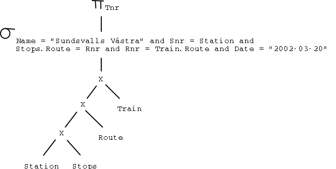
PROJECT_Tnr [ SELECT_{Name = "Sundsvalls Västra" and Snr = Station and Stops.Route = Rnr and Rnr = Train.Route and Date = "2002-03-20"} (Station X Stops X Route X Train) ]

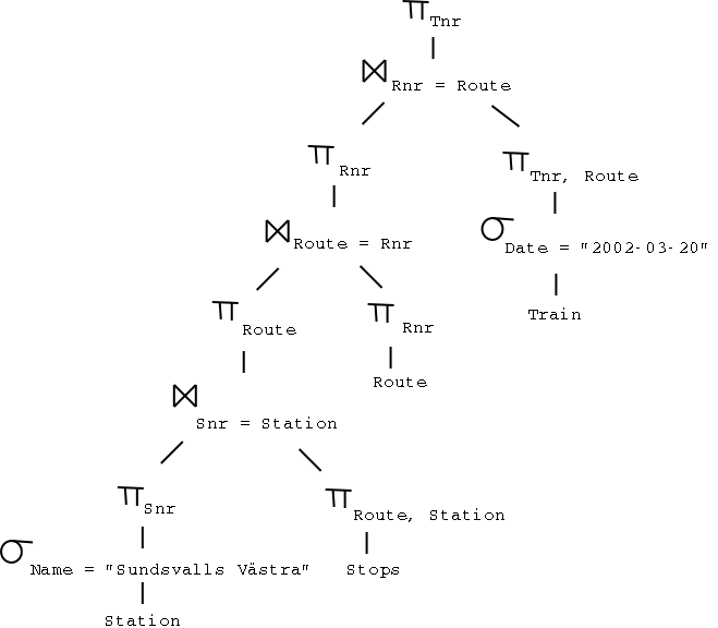
c)

Note: You can't remove the relation Route. Depending on the data in the database, a query with Route may give a different result compared to a query without. (But given certain referential integrity constraints, such an optimization may be possible.)

d)

Smaller intermediate results, with fewer tuples and fewer attributes, and therefore less work, since the optimized query tree

• performs select operations as early as possible
• uses joins, instead of Cartesian products followed by select operations
• (has re-orderered the relations to make joins possible)
• performs the most selective select operations first
• performs project operations as early as possible

e)

A heuristic query optimizer (of the type covered in this course) creates an execution plan by applying some general rules, such as "select operations should be performed as early as possible". It doesn't take into account different costs of using different algorithms for performing operations such as join and select. It doesn't take into account the size of the data, or the use of different physical storage structures (indexes).

A cost-based query optimizer, on the other hand, has a cost function, which is used to estimate the cost (typically measured in number of disk accesses) of an execution plan. To estimate the cost, the cost function must (and therefore does) take into account the actual or estimated size of the data, which storage structures exist, and also which algorithms will be used.

Problem 3

fsp <- RENAME_{(fsp_route, fsp_station, fsp_number, fsp_time)}(Stop)

lsp <- RENAME_{(lsp_route, lsp_station, lsp_number, lsp_time)}(Stop)

fsn <- RENAME_{(fsn_snr, fsn_name)}(Station)

lsn <- RENAME_{(fsn_snr, fsn_name)}(Station)

PROJECT_{fsp_time} ( SELECT_{fsn_name = "Sundsvalls Västra" and fsn_snr = fsp_station and fsp_route = Rnr and lsn_name = "Stockholms Central" and lsn_snr = lsp_station and lsp_route = Rnr and Rnr = Route and Date = "2002-03-20" and fsp_number < lsp_number} (fsn X lsn X fsp X lsp X Route X Train) )

A nicer solution:

fsp, lsp, fsn and lsn assigned as above

PROJECT_{fsp_time} ( SELECT_{fsp_number < lsp_number} [ (SELECT_{fsn_name = "Sundsvalls Västra"}(fsn)) JOIN_{fsn_snr = fsp_station} fsp JOIN_{fsp_route = Rnr} Route JOIN_{Rnr = lsp_route} lsp JOIN_{lsp_station = lsn_snr} (SELECT_{lsn_name = "Stockholms Central"}(lsn)) JOIN_{Rnr = Route} (SELECT_{Date = "2002-03-20"}(Train)) ] )

Problem 4

Use indexes on:

• Station.Snr
• Stops.Route
• Stops.Station
• Route.Rnr
• Train.Route
• Train.Date (used in select operations, and a large table, but perhaps low selectivity, and perhaps a wide column)

Also recommended:

• Station.Name (used in select operations, and has high selectivity, but a wide column and a fairly small table)
• Stops.Number (used, but for < and not =, and fairly low selectivity)

Not on:

• Stops.Time
• Route.Days
• Train.Tnr (unless just because it's the primary key)

Summary for grading:

Table	Should	Perhaps	Not
Station	Snr	Name
Stops	Route, Station	Number	Time
Route	Rnr		Days
Train	Route	Tnr, Date

Only Name, Date and Number: 1p

b)

• De-normalization.
• Pre-evaluated queries ("pre-evaluated views") stored in additional tables, possibly maintained by ECA rules in an active database.
• Use knowledge about the data to simplify queries, for example by removing the table Route from the query in problem 3.
• Buy faster hardware, or a faster DBMS.
• Wrong answer: Define views

Problem 5

a)

Heap. Record size = 4 + 4 + 10 = 18 bytes. Blocking factor bfr = 32768 / 18 = 1820. Number of blocks = 10⁶ / 1820 = 549. Since Tnr is a key, on an average we only need to read half the blocks, i. e. 274 blocks. 274 * 1 ms = 0.274 seconds.
Answer: 0.3 seconds.

b)

Primary B⁺ index. An index block has a fan-out of (32768 - 4) / (4 + 4) + 1 = 4096, and an "effective fan-out" of 2/3 * 4096 = 2730. Since this a primary index, assume that the records were inserted using that index, which gives an "effective bfr" in the data blocks of 2/3 * 1820 = 1213. Number of data blocks = 10⁶ / 1213 = 824. Since this is a primary index, it is enough with one pointer to each data block from the first index level. Number of blocks on first index level = 1213 / 824 = 2. Number of blocks on the second index level = 1. We have two index levels, and the data level. Required time = (2 + 1) * 10 ms = 30 ms.
Answer: 0.03 seconds.

c)

Secondary hash index. One lookup in the hash table (10 ms), and then one data block read (10 ms).
Answer: 0.02 seconds.

Alternative answers, using a block size of 1 kibibyte (1024) bytes: a) 9 seconds, b) 0.04 seconds, c) 0.02 seconds.

Problem 6

We need as many additional levels in the B⁺-tree index (problem 5b) that are required to handle 1000 sub-trees. With the 32-kibibyte blocks used in the example solution above, with an "effective fan-out" of 2730, one extra level is enough. (But since the level below the root was far from full in the example, actually no extra levels are needed.) With 1-kibibyte blocks, and an "effective fan-out" of 84, two extra levels are needed. (But since the level below the root was far from full in the example, actually only one extra level is needed.)
Short answer: The same time, plus between 0 and 0.02 seconds.

The execution time for the query using a secondary hash index (problem 5c) will be the same, 0.02 seconds. This assumes that the hash table is big enough. If the hash table was full from the start, and is not reorganized, this query may be much slower (in the worst case 1000 times slower, i. e. 20 seconds).
Short answer: The same time.

Problem 7

Normal index structures, such as B⁺ trees and hash tables, are one-dimensional, and can be used to quickly find a value on one axis. This makes them awkward for searches in two dimensions. You can use one of the dimensions for fast searches, but not the other. You can "fold" two dimensions into one by concatenating the values, but that doesn't help for searches on the second dimension. Compare with a phonebook sorted on last name and then first name: It is easy to find someone named "Andersson", but how do you find someone named "Bob" if you don't know his last name?

b)

Possible answers: K-d trees, K-d B-trees, quad trees, r-trees. Refer to the literature for a description of how they work.

Problem 8

a)

_NameF_count(*) ( SELECT_{Snr = Station} (Station X Stops) )

or

_NameF_count(*) ( Station JOIN_{Snr = Station} Stops )

b)

select Station.Name, count(Stops.Route)
from Station left outer join Stops on Station.Snr = Stops.Station
group by Station.Name

c)

_NameF_count(Route) ( Station LEFT OUTER JOIN_{Snr = Station} Stops )

Problem 9

Problem 10

a)

• Stops₁ = Stops SEMIJOIN_{Station = Snr} Station₁
• Stops₂ = Stops SEMIJOIN_{Station = Snr} Station₂
• Stops₃ = Stops SEMIJOIN_{Station = Snr} Station₃
• ...

b)

Station₁ UNION Station₂ UNION Station₃ UNION ...

c)

Stops₁ UNION Stops₂ UNION Stops₃ UNION ...

d) F_min(Time) ( [ SELECT_{Name = "Sundsvalls Central" and Country = "Sweden"} (Station) ] JOIN_{Snr = Station} Stops )

e)

F_min(Time) ( [ SELECT_{Name = "Sundsvalls Central" and Country = "Sweden"} (Station₁ UNION Station₂ UNION Station₃ UNION ...) ] JOIN_{Snr = Station} (Stops₁ UNION Stops₂ UNION Stops₃ UNION ...) )

f)

F_min(Time) ( [ SELECT_{Name = "Sundsvalls Central"} (Station₁) ] JOIN_{Snr = Station} Stops₁ )

Problem 11

Write locks give exclusive access to the locked resource, just as plain binary locks do. But several transactions can have read locks on the same resource at the same time, as long as no transaction has a write lock.
Wrong answer: Time stamps.

b)

To increase performance. Several transactions can have the data read-locked at the same time, instead of just one, which keeps the other transactions waiting.

c)

You might have several (local) copies of the (global, logical) data item that you want to lock. It is easy to lock one of the copies, but for global isolated (the I in ACID) transactions you need some sort of global locks that are made up of one or more local locks. (If, for example, a transaction could get a write lock on a single local copy, two transactions could write-lock two different copies, change them in different ways, and thus cause an inconsistency.)

There are several ways of creating a global lock out of one or more local locks.

• The primary copy method: On of the copies is designated the primary copy, and a local lock on that copy is equivalent to a global lock. (If all primary copies are stored at the same site, this can be called the primary site method.)
• Read locks one/write locks all: A local read lock on any of the copies is equivalent to a global read lock, but for a global write lock you need to local-write-lock all copies.
• Methods where you need to lock a certain number of local copies:
  • Majority locking, where you need a majority of the local read locks to get a global read lock, and a majority of the local write locks to get a global write lock
  • "k-of-n", where you need k local write locks (where n/2 < k <= n) to get a global write lock, and n - k + 1 local read locks to get a global read lock

Problem 12

The web server sends the SQL query string to the database server (using ODBC or some other interface). Typically, this is done without starting a separate program. Also, the web server can keep the connection to the database server open, and re-use the same session for all queries. The result is returned to the web server, which generates the HTML source code that is to be sent to the client.

b)

The main alternative is CGI scripts. A CGI script is a separate program, which is run by the web server. The output from the CGI script is sent to the client, and it is this output that is the web page that is shown to the user by the web browser. CGI scripts are usually written in a scripting language, such as Perl, but can also be a compiled program, written in a compiled language like C++ or Java.

CGI scripts are inefficient. Starting a new, separate program takes a long time on a computer. Also, if the CGI-generated web page contains output from a database, the CGI-script must open a new connection and log in on the database server, and this has to be done every time the web page is requested.